
Building a Multiplex from scratch with RWR_Make_Multiplex
Published:
In order to use any of the features of the RWRtoolkit package, you fill first need a multiplex network. A multiplex network is a topological construction of a series of networks. Instead of collapsing all networks into a single layer, a multiplex will instead maintain each layer’s distinct topology with edges existing between the same node within each layer (i.e. Node A existing in layer 1 will have edges to node A existing in layers 2, 3, and so on).
Setup for Constructing a Multiplex
In order to construct our multiplex, we first must create the individual layers (RWR_make_multiplex requires only that there exists edgelists of the layers. If you already have edgelists for you multiplex, please skip down to the next section). Below, we construct three separate layers, each with nodes and edges that exist in one, two, or all three layers. We then write those edges to a table file:
Layer Generation:
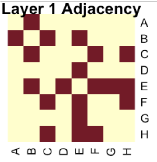
Layer 1
A◄───B◄──────C
     ▲       ▲
     │       │
D◄───E◄─┬──F─┤
     ▲  │  ▲ │
     │  │  │ │
 G───┘  H ─┴─┘
source <- c("B", "E", "C", "E", "F", "F", "G", "H", "H", "H")
sink <- c("A", "B", "B", "D", "E", "C", "E", "E", "F", "C")
weight <- rep(1, length(source))
edgelist <- matrix(c(source, sink, weight), ncol = 3, nrow = length(source))
colnames(edgelist) <- c("node1", "node2", "weight")
write.table(edgelist, "./abc_layer1.tsv", sep = "\t", row.names = FALSE, quote = FALSE)
| Source | Target | Weight |
|---|---|---|
| B | A | 1 |
| E | B | 1 |
| G | E | 1 |
| … | … | … |
graphtable <- read.table("./abc_layer1.tsv", sep = "\t", header = T)
layer1 <- igraph::graph_from_data_frame(graphtable, directed = F)
layer1_adj <- igraph::get.adjacency(layer1)
sorted_layer_names <- sort(row.names(layer1_adj))
sorted_adj <- layer1_adj[sorted_layer_names, sorted_layer_names]
stats::heatmap(as.matrix(sorted_adj)[nrow(as.matrix(sorted_adj)):1, ], Colv = NA, Rowv = NA, scale = "none", main = "Layer 1 Adjacency")
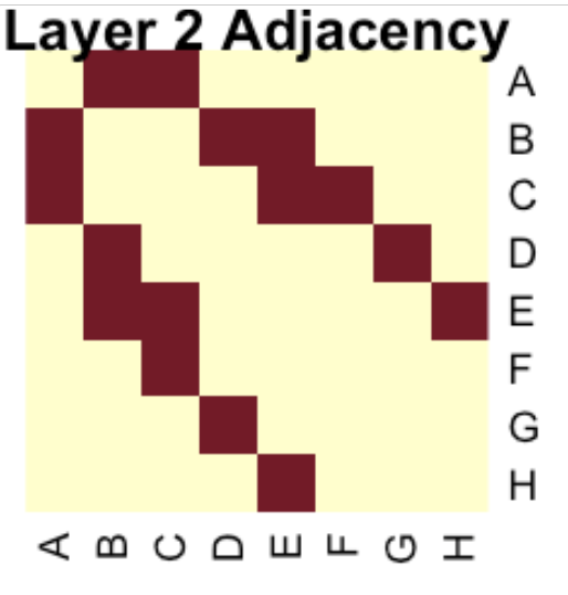
Layer 2
G        H
│        │
└──►D    └─►E       F
    │       │       │
    └───►B◄─┘──►C◄──┘
         │      │
         └──►A◄─┘
source <- c("G", "H", "D", "E", "F", "B", "C", "E")
sink <- c("D", "E", "B", "B", "C", "A", "A", "C")
weight <- rep(1, length(source))
edgelist <- matrix(c(source, sink, weight), ncol = 3, nrow = length(source))
colnames(edgelist) <- c("node1", "node2", "weight")
write.table(edgelist, "./abc_layer2.tsv", sep = "\t", row.names = FALSE, quote = FALSE)
| Source | Target | Weight |
|---|---|---|
| G | D | 1 |
| D | B | 1 |
| E | B | 1 |
| … | … | … |
graphtable <- read.table("./abc_layer2.tsv", sep = "\t", header = T)
layer2 <- igraph::graph_from_data_frame(graphtable, directed = F)
layer2_adj <- igraph::get.adjacency(layer2)
sorted_layer_names <- sort(row.names(layer2_adj))
sorted_adj <- layer2_adj[sorted_layer_names, sorted_layer_names]
stats::heatmap(as.matrix(sorted_adj)[nrow(as.matrix(sorted_adj)):1, ], Colv = NA, Rowv = NA, scale = "none", main = "Layer 2 Adjacency")
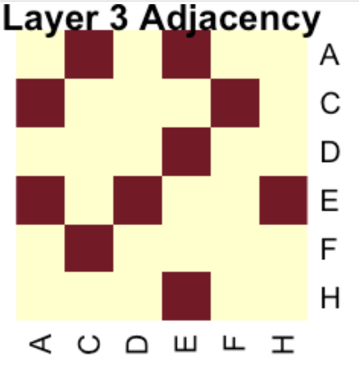
Layer 3
   H◄─┐
      │
 D◄───E◄┐        F
        │        │
        ├───►C◄──┘
        │
        A
source <- c("E", "E", "A", "A", "F")
sink <- c("H", "D", "E", "C", "C")
weight <- rep(1, length(source))
edgelist <- matrix(c(source, sink, weight), ncol = 3, nrow = length(source))
colnames(edgelist) <- c("node1", "node2", "weight")
write.table(edgelist, "./abc_layer3.tsv", sep = "\t", row.names = FALSE, quote = FALSE)
| Source | Target | Weight |
|---|---|---|
| E | H | 1 |
| E | D | 1 |
| A | E | 1 |
| … | … | … |
graphtable <- read.table("./abc_layer3.tsv", sep = "\t", header = T)
layer3 <- igraph::graph_from_data_frame(graphtable, directed = F)
layer3_adj <- igraph::get.adjacency(layer3)
sorted_layer_names <- sort(row.names(layer3_adj))
sorted_adj <- layer3_adj[sorted_layer_names, sorted_layer_names]
stats::heatmap(as.matrix(sorted_adj)[nrow(as.matrix(sorted_adj)):1, ], Colv = NA, Rowv = NA, scale = "none", main = "Layer 3 Adjacency")
FLIST Generation
We now have all three of our layers, we need to create a file that describes:
- Where our layers live
- What our layers are called
| File Path | Short Name |
|---|---|
| path_to_file1 | layer1_name |
| path_to_file2 | layer2_name |
| path_to_file3 | layer3_name |
filepaths <- c("./abc_layer1.tsv", "./abc_layer2.tsv", "./abc_layer3.tsv")
layernames <- c("layer1", "layer2", "layer3")
flist_df <- data.frame(list(filepaths = filepaths, layernames = layernames))

flist_filename <- "multiplex_flist.tsv"
write.table(flist_df, file = flist_filename, quote = F, sep = "\t", row.names = F, col.names = F)
Constructing a Multiplex Network:
Now that we have our multiplex flist generated above, we can make a multiplex with RWR_make_multiplex. Depending on how large your layers are, this can be a rate limiting step.
multiplex_filename <- "abc_multiplex.Rdata"
RWR_make_multiplex(flist_filename, output = multiplex_filename)

# load saved data:
load(multiplex_filename)
Currently RWR_make_multiplex saves the networks to file for easier access in the future. The data saved within the file are:
nw.mpo: An object containing:Number of Layers: The total number of layers within the multiplex network.Number of Nodes: Total number of nodes within the network (not including duplicates of nodes between layers).Pool of Nodes: A comprehensive list of all nodes within the entire multiplex network.- Individual Layers: Distinct igraph object layers.
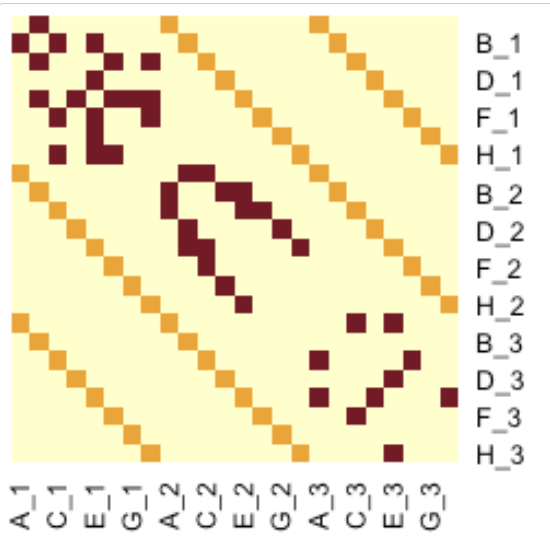
nw.adj: A supra-adjacency matrix in which all layers occur along the diagonal and inter-layer edges occur on the off diagonal. In the below image, we can see that the topologies of each particular layer are maintained within the supra-adjacency matrix along the diagonal:
# Reversed matrix as stats heatmap plots rows in reverse order.
stats::heatmap(as.matrix(nw.adj)[nrow(as.matrix(nw.adj)):1, ], Colv = NA, Rowv = NA, scale = "none")
nw.adjnorm: Similar to the above, thenw.adjnormtakes the abovenw.adjmatrix and normalizes colum-nwise such that each column sums to 1 and each edge has a $\frac{1}{D( A_{i,j} )}$ probability of being walked by the random walker.
stats::heatmap(as.matrix(nw.adjnorm)[nrow(as.matrix(nw.adjnorm)):1, ], Colv = NA, Rowv = NA, scale = "none")
![]()
No we have made our multiplex and are ready to run any of the tools within the RWRtoolkit!