
Using RWR_shortest_paths between Seed Sets to Explore Multiplex Connectivity
Published:
With Shortest Paths the shortest paths function, we generate a list of the shortest paths between two vertices ordered by the number of nodes traversed. Not only may any two vertices be supplied as potential source and target nodes, but entire sets may be supplied as well.
1. Introduction
In a given multiplex, there are a number of paths of equal lengths between any two nodes. The RWR_ShortestPaths function calculates the shortest paths between any two nodes, and includes associated node weights for each particular layer in which that path exists.
2. Setup
Layer Generation
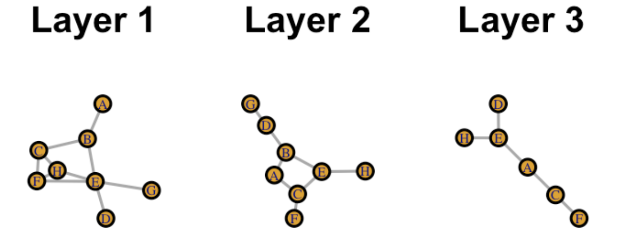
The RWR_ShortestPaths function requres an mpo R object (generated from RWR_make_multiplex), a vector of source nodes and a vector of target nodes. First we’ll need to create an example multiplex. In this example, we’ll create a 3 layer multiplex:
library(RWRtoolkit)
library(igraph)

# Layer 1
source <- c("B", "E", "C", "E", "F", "F", "G", "H", "H", "H")
sink <- c("A", "B", "B", "D", "E", "C", "E", "E", "F", "C")
weight <- rep(1, length(source))
edgelist_layer1 <- data.frame(list(source = source, sink = sink, weight = weight))
write.table(edgelist_layer1, "./abc_layer1.tsv", sep = "\t", row.names = FALSE, quote = FALSE)

# Layer 2
source <- c("G", "H", "D", "E", "F", "B", "C", "E")
sink <- c("D", "E", "B", "B", "C", "A", "A", "C")
weight <- rep(1, length(source))
edgelist_layer2 <- data.frame(list(source = source, sink = sink, weight = weight))
write.table(edgelist_layer2, "./abc_layer2.tsv", sep = "\t", row.names = FALSE, quote = FALSE)

# Layer 3
source <- c("E", "E", "A", "A", "F")
sink <- c("H", "D", "E", "C", "C")
weight <- rep(integer(1), length(source))
edgelist_layer3 <- data.frame(list(source = source, sink = sink, weight = weight))
write.table(edgelist_layer3, "./abc_layer3.tsv", sep = "\t", row.names = FALSE, quote = FALSE)
To generate a figure for the above layers, use the following code:
set.seed(32)
layer1 <- igraph::graph_from_data_frame(edgelist_layer1, directed= F)
layer2 <- igraph::graph_from_data_frame(edgelist_layer2, directed= F)
layer3 <- igraph::graph_from_data_frame(edgelist_layer3, directed= F)
output <- capture.output({
  V(layer1)$label.cex <- 0.45
  V(layer2)$label.cex <- 0.45
  V(layer3)$label.cex <- 0.45

  png('layers.png', width=700, height=350, res=300)
  par(mfrow= c(1,3), mar=c(1,1,1,1))
  igraph::plot.igraph(layer1, main="Layer 1", vertex.size=28)
  igraph::plot.igraph(layer2, main="Layer 2", vertex.size=28)
  igraph::plot.igraph(layer3, main="Layer 3", vertex.size=28)
  dev.off()
})
knitr::include_graphics('layers.png')
FLIST and Multiplex Generation
We now have all three of our layers, we need to create a quick flist and then to make our multiplex! The flist must be a file of the type:
| File Path | Short Name | Group |
|---|---|---|
| path_to_file1 | layer1_name | layer_group |
| path_to_file2 | layer2_name | layer_group |
| path_to_file3 | layer3_name | layer_group |
And once we have our multiplex flist, we can make a multiplex with RWR_make_multiplex:
filepaths <- c("./abc_layer1.tsv", "./abc_layer2.tsv", "./abc_layer3.tsv")
layernames <- c("layer1", "layer2", "layer3")
groups <- c(1, 1, 1)
flist_df <- data.frame(list(filepaths = filepaths, layernames = layernames, groups = groups))


flist_filename <- "multiplex_flist.tsv"
write.table(flist_df, file = flist_filename, quote = F, sep = "\t", row.names = F, col.names = F)

multiplex_filename <- "abc_multiplex.Rdata"
RWR_make_multiplex(flist_filename, output = multiplex_filename)

# load saved data:
load(multiplex_filename)
Node Set Generation
Now that we have our multiplex, let’s use RWR_shortestpaths to extract some information!
It should be noted that RWR_ShortestPaths can be run in two separate modes:
With only
source_genesetsuch that shortest paths will be generated between all named nodes within the list.With both
source_genesetandtarget_genesetsuch that all shortest paths will be found between each node within thesource_genesetto each target node in thetarget_geneset.
Additionally, it ought to be noted that all provided geneset files ought to be formatted in a way such that there exist two columns, the first being setid the second being the corresponding node in the network (gene), such as:
| Set ID | Node Name |
|---|---|
| setA1 | A |
| setA1 | C |
| setA1 | G |
| setA1 | F |
Let’s extract our first path to be a path from nodes G to C. To do so, we’ll need a target file and a source file, each consisting of a list of nodes with an associated set name).
source_nodes <- c("G")
target_nodes <- c("C")

node_sets <- c("set1")

source_list <- list(set = node_sets, node = source_nodes)
target_list <- list(set = node_sets, node = target_nodes)

source_df <- data.frame(source_list)
target_df <- data.frame(target_list)

source_file <- "source_G.tsv"
target_file <- "target_C.tsv"

write.table(source_df, file = source_file, quote = F, sep = "\t", row.names = F, col.names = F)
write.table(target_df, file = target_file, quote = F, sep = "\t", row.names = F, col.names = F)
Running RWR_ShortestPaths
Finally, now that we have a network, source nodes, and target nodes, we can call RWR_shortestpaths.
shortest_paths_output <- RWRtoolkit::RWR_ShortestPaths(
  data = multiplex_filename,
  source_geneset = source_file,
  target_geneset = target_file
)

shortest_paths_output
#>   from to weight   type weightnorm pathname pathlength pathelements
#> 1    E  C      1 layer2      0.125      G_C          3      G->E->C
#> 2    E  G      1 layer1      0.100      G_C          3      G->E->C
In the above dataframe, between each combination of the elements within geneset1 and geneset2. Each row corresponds to a given link in a path from one gene to another with:
- Corresponding edge weight from their original layers
- A normlalized weight with respect to each layer (i.e. all edges within the layer have been normalized such that the sum of all edge weights within the layer sum to 1).
- The layer from which the edge came.
- A distinct pathname with respect to the starting element and ending element
- Path Length
- A full path for all nodes.
Note, given that RWR Toolkit does not currently employ methods for directed networks, the directionality of the from and to columns may not align with the directionality of the pathelements column.
In the above example output, we see that the two layers in which our shortest path from G to A exist are layers 1 and 2. It is not always the case that only one path will exist in a dataset, however. This can be illustrated with by obtaining the shortest paths from H to A:
source_nodes <- c("H")
target_nodes <- c("A")

node_sets <- c("set1")

source_list <- list(set = node_sets, node = source_nodes)
target_list <- list(set = node_sets, node = target_nodes)

source_df <- data.frame(source_list)
target_df <- data.frame(target_list)

source_file <- "source_H.tsv"
target_file <- "target_A.tsv"

write.table(source_df, file = source_file, quote = F, sep = "\t", row.names = F, col.names = F)
write.table(target_df, file = target_file, quote = F, sep = "\t", row.names = F, col.names = F)

shortest_paths_output <- RWRtoolkit::RWR_ShortestPaths(
  data = multiplex_filename,
  source_geneset = source_file,
  target_geneset = target_file
)

shortest_paths_output
#>   from to weight   type weightnorm pathname pathlength pathelements
#> 1    E  H      1 layer3      0.200      H_A          3      H->E->A
#> 2    E  H      1 layer2      0.125      H_A          3      H->E->A
#> 3    E  H      1 layer1      0.100      H_A          3      H->E->A
#> 4    E  A      1 layer3      0.200      H_A          3      H->E->A
In the above output, we have two options for the edge that exists between nodes H and E. We can use RWRtoolkit::extract_highest_scoring_path in order to obtain the highest scoring path of our path. This does so by extracting the edges with the highest weight either by weight or by weightnorm (defaulted).
desired_path <- "H_A"
optimal_paths <- RWRtoolkit::extract_highest_scoring_path(shortest_paths_output, desired_path)

optimal_paths
#>   from to weight   type weightnorm pathname pathlength pathelements
#> 1    H  E      1 layer3        0.2      H_A          3      H->E->A
#> 4    E  A      1 layer3        0.2      H_A          3      H->E->A
Using Real Data
In order to deomonstrate RWR_ShortestPaths on a more realistic data set, we will start with a predefined network from the package (any Rdata object created from the RWR_make_multiplex function will suffice). The string_interactions.Rdata network
Load the Network
extdata.dir <- system.file("example_data", package = "RWRtoolkit")
multiplex_object_filepath <- paste(extdata.dir, "/string_interactions.Rdata", sep = "")
The string_interaction multiplex contains 9 layers:
| Layer Number | Layer Name | Edge Count |
|---|---|---|
| 1 | Automated Textmining | 160 |
| 2 | Coexpression | 154 |
| 3 | Combined Score | 162 |
| 4 | Database Annotated | 136 |
| 5 | Experimentally Determined Interaction | 71 |
| 6 | Gene Fusion | 5 |
| 7 | Homology | 13 |
| 8 | Neighborhood on Chromosome | 87 |
| 9 | Phylogenetic Cooccurrence | 20 |
Load the Two Gene Sets
Next we must define the geneset paths from which to define our source and target nodes. Only the file paths are needed for the genesets:
geneset1_filepath <- paste(extdata.dir, "/geneset1.tsv", sep = "")
geneset2_filepath <- paste(extdata.dir, "/geneset2.tsv", sep = "")
outdir <- paste(extdata.dir, "/out/rwr_shortestpath", sep = "")
Geneset 1
| Set ID | Node Name |
|---|---|
| setA1 | G6PD |
| setA1 | PMM1 |
| setA1 | TPI1 |
| setA1 | PFKM |
| setA1 | HKDC1 |
| setA1 | CDC5L |
| setA1 | ENO1 |
| setA1 | ENO3 |
| setA1 | GAPDH |
| setA1 | GCK |
| setA1 | GFPT1 |
| setA1 | PKLR |
Geneset 2
| Set ID | Node Name |
|---|---|
| setA2 | PGLS |
| setA2 | PMM2 |
| setA2 | PKLR |
| setA2 | HK3 |
| setA2 | HK2 |
3. Running RWR_ShortestPaths
To run RWR Shortest Paths we paste in the filepaths to our flist, source, and target genesets:
shortest_path_df <- RWR_ShortestPaths(
  data = multiplex_object_filepath,
  source_geneset = geneset1_filepath,
  target_geneset = geneset2_filepath
)

head(shortest_path_df)
#>   from  to     weight                 type  weightnorm pathname pathlength
#> 1 G6PD HK2 0.88888889   database_annotated 0.006916825 G6PD_HK2          2
#> 2 G6PD HK2 0.95595596       combined_score 0.006180630 G6PD_HK2          2
#> 3 G6PD HK2 0.09869848         coexpression 0.002553311 G6PD_HK2          2
#> 4 G6PD HK2 0.80082559 automated_textmining 0.007730624 G6PD_HK2          2
#> 5 G6PD HK3 0.88888889   database_annotated 0.006916825 G6PD_HK3          2
#> 6 G6PD HK3 0.90190190       combined_score 0.005831149 G6PD_HK3          2
#>   pathelements
#> 1    G6PD->HK2
#> 2    G6PD->HK2
#> 3    G6PD->HK2
#> 4    G6PD->HK2
#> 5    G6PD->HK3
#> 6    G6PD->HK3
Once you have obtained the shortest paths results, we can either view all edges within a shortest path, such as:
shortest_path_df[shortest_path_df$pathname == "PMM1_PGLS", ]
#>    from   to     weight                       type  weightnorm  pathname
#> 36 H6PD  HK1 0.88888889         database_annotated 0.006916825 PMM1_PGLS
#> 37 H6PD  HK1 0.96796797             combined_score 0.006258292 PMM1_PGLS
#> 38 H6PD  HK1 0.16268980               coexpression 0.004208754 PMM1_PGLS
#> 39 H6PD  HK1 0.84726522       automated_textmining 0.008178920 PMM1_PGLS
#> 40 H6PD PGLS 0.72383073  phylogenetic_cooccurrence 0.041709446 PMM1_PGLS
#> 41 H6PD PGLS 0.30578512 neighborhood_on_chromosome 0.007920651 PMM1_PGLS
#> 42 H6PD PGLS 0.74847251                   homology 0.060454022 PMM1_PGLS
#> 43 H6PD PGLS 1.00000000         database_annotated 0.007781428 PMM1_PGLS
#> 44 H6PD PGLS 0.93893894             combined_score 0.006070608 PMM1_PGLS
#> 45 H6PD PGLS 0.14642082               coexpression 0.003787879 PMM1_PGLS
#> 46 H6PD PGLS 0.79979360       automated_textmining 0.007720661 PMM1_PGLS
#> 47  HK1 PMM1 1.00000000         database_annotated 0.007781428 PMM1_PGLS
#> 48  HK1 PMM1 0.91391391             combined_score 0.005908811 PMM1_PGLS
#> 49  HK1 PMM1 0.06616052               coexpression 0.001711560 PMM1_PGLS
#> 50  HK1 PMM1 0.15273478       automated_textmining 0.001474397 PMM1_PGLS
#>    pathlength          pathelements
#> 36          4 PMM1->HK1->H6PD->PGLS
#> 37          4 PMM1->HK1->H6PD->PGLS
#> 38          4 PMM1->HK1->H6PD->PGLS
#> 39          4 PMM1->HK1->H6PD->PGLS
#> 40          4 PMM1->HK1->H6PD->PGLS
#> 41          4 PMM1->HK1->H6PD->PGLS
#> 42          4 PMM1->HK1->H6PD->PGLS
#> 43          4 PMM1->HK1->H6PD->PGLS
#> 44          4 PMM1->HK1->H6PD->PGLS
#> 45          4 PMM1->HK1->H6PD->PGLS
#> 46          4 PMM1->HK1->H6PD->PGLS
#> 47          4 PMM1->HK1->H6PD->PGLS
#> 48          4 PMM1->HK1->H6PD->PGLS
#> 49          4 PMM1->HK1->H6PD->PGLS
#> 50          4 PMM1->HK1->H6PD->PGLS
Or we extract the shortest path with the highest edge weights:
desired_path <- "PMM1_PGLS"
optimal_paths <- RWRtoolkit::extract_highest_scoring_path(shortest_path_df, desired_path)

optimal_paths
#>    from   to   weight               type  weightnorm  pathname pathlength
#> 47 PMM1  HK1 1.000000 database_annotated 0.007781428 PMM1_PGLS          4
#> 37  HK1 H6PD 0.967968     combined_score 0.006258292 PMM1_PGLS          4
#> 43 H6PD PGLS 1.000000 database_annotated 0.007781428 PMM1_PGLS          4
#>             pathelements
#> 47 PMM1->HK1->H6PD->PGLS
#> 37 PMM1->HK1->H6PD->PGLS
#> 43 PMM1->HK1->H6PD->PGLS