
Seed Set Connectivity Calculations with RWR_CV
Published:
This vignette descibes the usage of RWR_CV with respect to differing gene sets and the parsing of RWR_CV’s output.
This method can be used in two ways:
- Using an independently curated set of well connected genes to score a newly generated multiplex.
- Using a well generated multiplex to explore seed set connectivity.
In this vignette, we will be exploring the second method. To run this algorithm, we will need a multiplex object and a gene set.
The predictive ability of a multiplex network can be determined using cross validation of gold standard gene sets with the RWR_CV command. A gold standard gene set typically contains genes that are known to be functionally related (for example all are members of one biosynthetic pathway, or all are annotated with the same GO term). In theory, if only some members of the gold set are used as seeds, those that were left out should be found with relatively high precision (i.e. highly ranked by RWR) if the underlying networks are indeed functionally predictive.
The RWR_CV command allows the user to provide a gold gene set and use k-fold, leave-one-out, or singleton cross validation. Metrics such as AUROC and AUPRC are provided, also in the form of plots, in order for the user to determine if their multiplex network is truly predictive. If a multiplex network were constructed from layers containing entirely random edges between genes, then the expectation would be AUROC = 0.50 and AUPRC = g/n where g is the size of the gene set and n is the number of unique genes in the multiplex. If RWR_CV shows higher values than these with multiple gold gene sets, this indicates a functionally useful biological multiplex.
Just as gold gene sets can be used to evaluate a multiplex network, the multiplex network can be used to evaluate a user’s gene set via cross-validation. In this scenario it is assumed that the underlying network contains true functional links between genes. If the genes in the geneset are functionally related then the seed genes should find the left out (validation) genes with high ranks. On the other hand, if the geneset is unrelated then the seed genes will be no more useful than random genes for finding the validation genes.
Four output files are generated by the running of RWR_CV are:
- The full ranks file gives the ranks obtained from each particular fold of the cross validation in addition to output statistics.
- The mean ranks file: contains the mean rank for each ranked node across each fold. For example, from the example command output, gene PFKP is of rank 2 in the first 2 folds, yet rank 17 in the third fold. While PFKP enjoys the rank of 2 in two of the three folds, it would be spurious to discount the fold in which PFKP’s rank is 17. By taking the mean of the ranks across all folds, a more generic scoring metric can be obtained. Note, if there exist any ties within the mean ranks, the rerank column denotes consecutive ranks with respect to those ties.
- The metrics file: is comprised of metrics for all mean ranked genes denoting True Positive (TP) (i.e. ranked genes in the supplied geneset), False Positive (FP) (ranked genes that do not exist within the geneset), Cumulative TP and FP as ranks increase, False Positive Rate (i.e. the cumulative number of false positives at row i over the total number of ranked genes), Precision, and Recall.
- The summary file: contains summary statistics for each particular fold and the mean of the folds. For each fold, values are reported for varying measures such as Average Precision, AUROC, AUPRC.
2. Setup
In order to run RWR_CV, we will need an mpo object. These are derived from the RWRtoolkit::RWR_make_multiplex function. For this vignette, we will use previously defined multiplex objects.
Obtaining the Networks
Downloading a multiplex network:
library(RWRtoolkit)
We’ll select an A. thaliana multiplex consisting of 10 layers (for further description of each layer, please click the associated link):
| Network | Nodes | Edges |
|---|---|---|
| CoEvolution-DUO (DU) version 0.1 | 2,283 | 13,514 |
| Coexpression Gene-Atlas (GA) version 0.3 | 7,683 | 84,959 |
| Knockout Similarity (KS) version 0.3 | 1,841 | 94,952 |
| PPI-6merged (PP) version 0.3 | 19,191 | 317,787 |
| PEN-Diversity (PX) version 0.1 | 17,907 | 97,819 |
| Predictive CG Methylation (PY) version 0.1 | 13,314 | 76,027 |
| Regulation-ATRM (RE) version 0.3 | 789 | 1,359 |
| Regulation-Plantregmap (RP) version 0.3 | 16,014 | 167,851 |
| Metabolic-AraCyc (RX) version 0.3 | 2,857 | 21,524 |
athal_multiplex_url <- "https://github.com/dkainer/RWRtoolkit-data/raw/main/Comprehensive_Network_AT_d0.5_v02.RData?raw=True"
athal_multiplex <- url(athal_multiplex_url)
load(athal_multiplex)

athal_multiplex_object <- nw.mpo
athal_multiplex_adj <- nw.adj
athal_multiplex_transmat <- nw.adjnorm
Building a “Gold Set”
We will need a “gold set” of genes to test our multiplex network against. These “gold standard” genes are ones that are previously defined as being highly related in some fashion (e.g. genes with the same GO or Mapman description).
For our “gold set” of genes, we will use the well described and highly conserved Jasmonte pathway genes defined by MapMan (Table S1). We will then need to annotate those genes with a “set”, as goldset files follow the format (where the set name is some defining string and the gene ids are strings that match to node names within the multiplex):
| Set Name | Gene ID |
|---|---|
| goldSet | node1 |
| goldSet | node2 |
| goldSet | node3 |
| goldSet | node4 |
We can create our own gold set file with:
# Define Genes
jasmonate_seed_genes <- c(
	"AT2G44810", "AT1G17420", "AT1G55020", "AT1G67560",
	"AT1G72520", "AT3G22400", "AT3G45140", "AT5G42650",
	"AT1G13280", "AT3G25760", "AT3G25770", "AT3G25780",
	"AT1G09400", "AT1G17990", "AT1G18020", "AT1G76680",
	"AT1G76690", "AT2G06050", "AT1G17380", "AT1G19180",
	"AT1G48500", "AT1G70700", "AT1G72450", "AT1G74950",
	"AT3G17860", "AT3G43440", "AT5G20900"
)
# Add annotations
seed_gene_setname <- rep("jasmonate_mm", length(jasmonate_seed_genes))
seed_gene_df <- data.frame("set" = seed_gene_setname, "seed" = jasmonate_seed_genes)

# Write File
goldset_filename <- "./goldset_jasomonate.tsv"
write.table(seed_gene_df, goldset_filename, sep = "\t", row.names = FALSE, col.names = FALSE, quote = FALSE)
Building a “Bronze Set”
For the sake of illustration, we will generate a set with partially connected, and partially randomly sampled genes, which we will refer to as the “bronze set”.
The general idea behind creating this bronze set is to illustrate how scoring works with respect to a set of genes that are not well connected within the supplied network.
We have built our gold set of Jasmonate MapMan described genes above. We will now replace genes known to be related within the Jasmonate description with others randomly sampled within the network:
# Replace 60% of Jasmonate genes with randomly sampled genes
set.seed(42)
`%notin%` <- Negate(`%in%`)

newly_sampled_percentage <- 2 / 3
n_genes_for_sampling <- floor(length(jasmonate_seed_genes) * newly_sampled_percentage)

gene_pool <- athal_multiplex_object$Pool_of_Nodes[ athal_multiplex_object$Pool_of_Nodes %notin% jasmonate_seed_genes ]

random_sample <- sample(gene_pool, replace = FALSE, size = n_genes_for_sampling)

## Replace:
seed_gene_df$seed[1:length(random_sample)] <- random_sample

random_sample_filename <- "./partially_random_sample_seeds.tsv"
write.table(seed_gene_df, random_sample_filename, row.names = FALSE, col.names = FALSE, quote = FALSE)
We now have two sets of genes: one in which there exists known connections between all genes within the set, and another with known connections between only $\frac{1}{3}$ of the genes. Running RWR_CV for both our gold set and our bronze set, we can then compare the outputs.
Runing RWR CV
When running RWR_CV, there exist multiple methods in which to test the gene sets with respect to the networks. Users have the ability to select a method of either:
KFold: Each relevant gene R is ranked K times (as there are K folds), resulting in $\sum R$ / K mean fold scores per gene R.
Leave One Out (LOO): Each relevant gene R is ranked once in that there are R total folds, with 1 gene left out per fold.
Singletons: Each relevant gene R is ranked $R-1$ times. There are R folds, with $R-1$ left out per fold.
Given the nature of how each method works, the above methods do have differing outputs:
For each of these, scoring metrics are then used to generate the final tables consisting of:
fullranks: These data include the ranks for each particular fold within the k folds for each node within the network.metrics: These data include the information frommedianrankson top of:True positive (TP): that is, are the ranked genes within median ranks members of the provided gene set
False positive (FP): Genes that exist within the top median ranked genes, yet not in the provided gene set
True Negative: TN
False Negative: FN
Cumulative Scores for TP / FP / TN / FN as ranks increase.
False Positive Rate (FPR): The cumulative false positive for at row i over the total number of false positives.
Precision: True Positive / ( True Positive + False Positive)
Recall: True Positive / (True Positive + False Negative)
summary: The Summary of the k fold output contains:Fold: The associated fold
Value: The Value of the function noted in
measureMeasure:
P@NumLeftOut: Percentage of the number of genes left outAvgPrec: Average Precision.
Geneset: The geneset of the associated input genes.
kFold
With our multiplex, gold and bronze set genes in place, we can run RWR_CV. First, let’s run kfold on the gold set genes to see how well they perform. By using the kfold method, genes are randomly split into groups of seeds to see how well those seed groups can recall the left out genes:
gold_path <- "goldset_kfold_output"
gold_cv_kfold_output <- RWRtoolkit::RWR_CV(
  data = athal_multiplex_url,
  geneset_path = goldset_filename,
  method = "kfold",
  write_to_file=TRUE,
  plot = TRUE,
  outdir = gold_path
)

bronze_path <- "bronzeset_kfold_output"
bronze_cv_kfold_output <- RWRtoolkit::RWR_CV(
  data = athal_multiplex_url,
  geneset_path = random_sample_filename,
  method = "kfold",
  write_to_file=TRUE,
  plot = TRUE,
  outdir = bronze_path)
RWR_CV Kfold Output Analysis
After running the above two functions, we can see the main difference between the two gene sets in their output metrics:
Gold Set
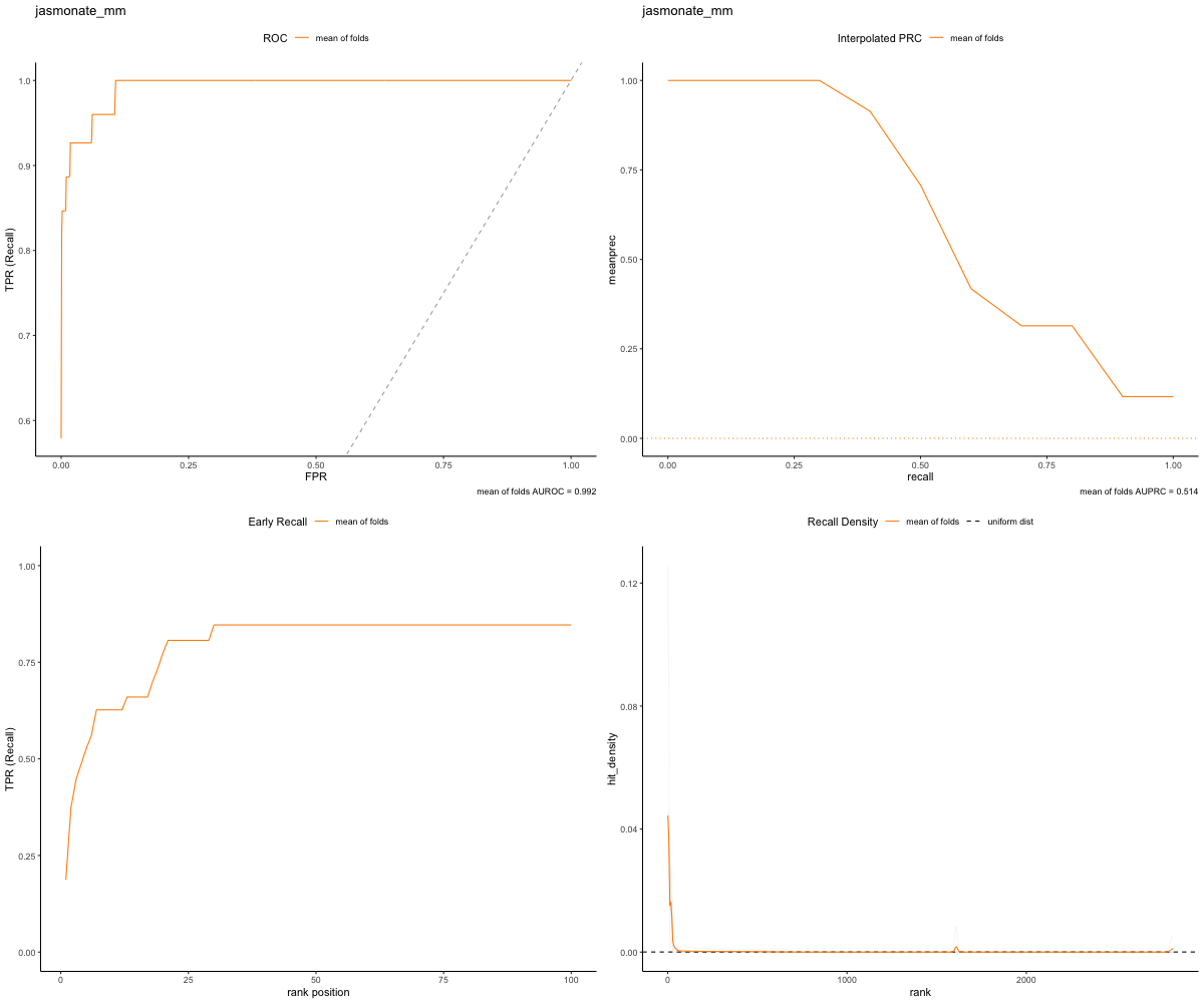
head(gold_cv_kfold_output$metrics)
In the gold set run, when initially viewing the head of the dataframe, we can see that the top ranked genes from our network are in the validation set of gene (resulting in true positive matches). Additionally, upon visual inspection of the plots, we can see that our ROC curve quickly ranks all genes within the network!
image_path <- paste(gold_path, "RWR-CV_jasmonate_mm_Comprehensive_Network_AT_d0.5_v02_default.plots.png", sep="/")

knitr::include_graphics(image_path)
Bronze Set
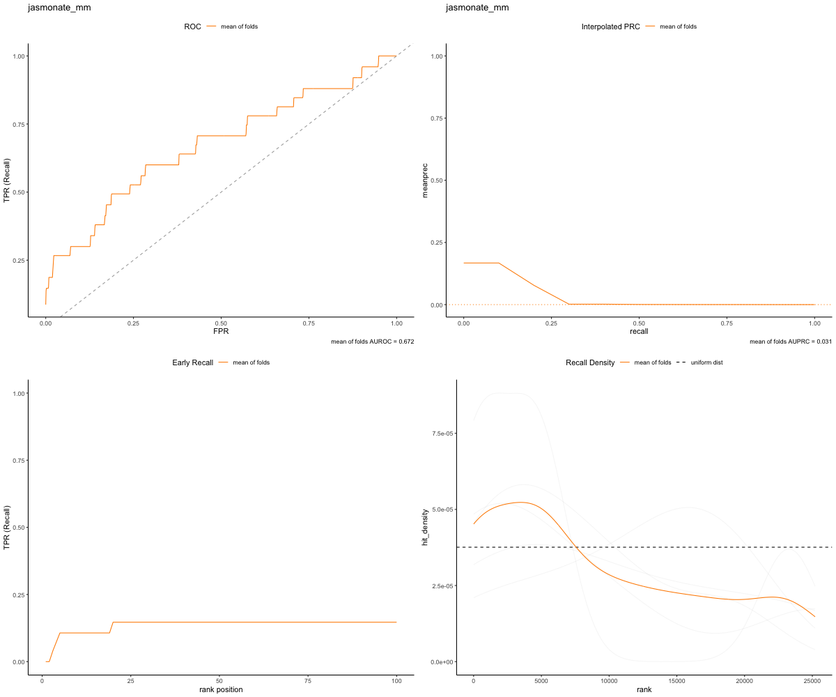
head(bronze_cv_kfold_output$metrics)
Notice that the Bronze Set , however, our top ranked genes have no true positives. The bronze set has significantly fewer True Positive matches than does the Gold Set. That means that as the random walker traversed the network, it took quite a while to recall the other genes within the set. Additionally this can be illustrated by the plot below:
image_path <- paste(bronze_path, "RWR-CV_jasmonate_mm_Comprehensive_Network_AT_d0.5_v02_default.plots.png", sep="/")

knitr::include_graphics(image_path)
Leave One Out
Instead of randomly shuffling the gene set k times for a train/test split, we can remove only one gene from the gene set and see how quickly the random walker can recall that gene. This is done for every gene within the genes set, so if there exist N genes, we will run a random walk N times:
gold_path <- "goldset_loo_output"
gold_cv_loo_output <- RWRtoolkit::RWR_CV(
  data = athal_multiplex_url,
  geneset_path = goldset_filename,
  method = "loo",
  write_to_file=TRUE,
  plot = TRUE,
  outdir = gold_path
)

bronze_path <- "bronzeset_loo_output"
bronze_cv_loo_output <- RWRtoolkit::RWR_CV(
  data = athal_multiplex_url,
  geneset_path = random_sample_filename,
  method = "loo",
  write_to_file=TRUE,
  plot = TRUE,
  outdir = bronze_path)
RWR_CV LOO Output Analysis
Now, instead of using our method of separation as kfold, we can leave only 1 node out using LOO:
Gold Set
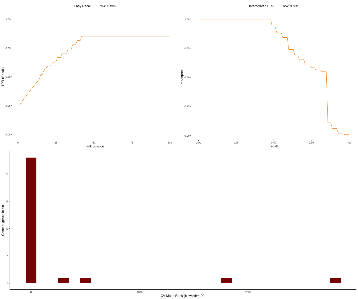
head(gold_cv_loo_output$metrics)
Similarly to the above output for kfold, we can see that the top ranked genes in the goldset run from our network are in the validation set of genes, resulting in more true positives:
image_path <- paste(gold_path, "RWR-CV_jasmonate_mm_Comprehensive_Network_AT_d0.5_v02_default.plots.png", sep="/")

knitr::include_graphics(image_path)
Bronze Set
head(bronze_cv_loo_output$metrics)
Notice that between on the other hand, however, our top ranked genes have no true positives. The bronze set has significantly fewer True Positive matches than does the Gold Set. Additionally this can be illustrated by the plot below:
image_path <- paste(bronze_path, "RWR-CV_jasmonate_mm_Comprehensive_Network_AT_d0.5_v02_default.plots.png", sep="/")

knitr::include_graphics(image_path)

Singletons
With our method of separation being “singletons”, we leave out all nodes except for 1, and see how well that single node can recall the others within the set:
gold_path <- "goldset_singleton_output"
gold_cv_singleton_output <- RWRtoolkit::RWR_CV(
  data = athal_multiplex_url,
  geneset_path = goldset_filename,
  method = "singletons",
  write_to_file=TRUE,
  plot = TRUE,
  outdir = gold_path
)

bronze_path <- "bronzeset_singleton_output"
bronze_cv_singleton_output <- RWRtoolkit::RWR_CV(
  data = athal_multiplex_url,
  geneset_path = random_sample_filename,
  method = "singletons",
  write_to_file=TRUE,
  plot = TRUE,
  outdir = bronze_path)
RWR_CV singleton Output Analysis
Gold Set
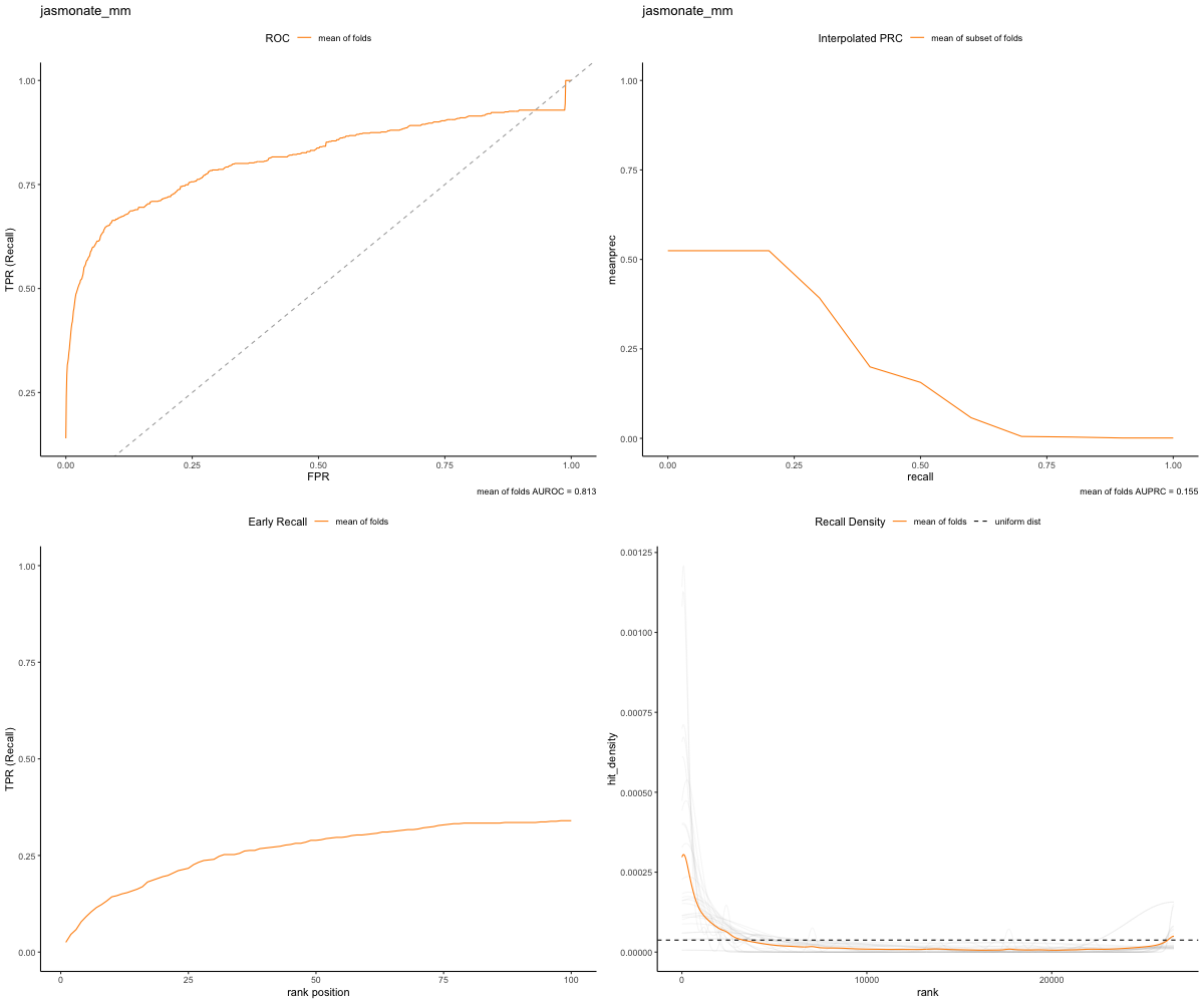
head(gold_cv_singleton_output$metrics)
In the gold set run, we can see that the top ranked genes from our network are in the validation set of genes, resulting in more true positives:
image_path <- paste(gold_path, "RWR-CV_jasmonate_mm_Comprehensive_Network_AT_d0.5_v02_default.plots.png", sep="/")

knitr::include_graphics(image_path)
Bronze Set
head(bronze_cv_singleton_output$metrics)
Notice that between on the other hand, however, our top ranked genes have no true positives. The bronze set has significantly fewer True Positive matches than does the Gold Set. Additionally this can be illustrated by the plot below:
image_path <- paste(bronze_path, "RWR-CV_jasmonate_mm_Comprehensive_Network_AT_d0.5_v02_default.plots.png", sep="/")

knitr::include_graphics(image_path)
